This study is focused on the complex terrain region around the Biglow Canyon wind farm. It is located in the region near the second Wind Forecast Improvement Project (WFIP2) site, characterized by pronounced topographic features.
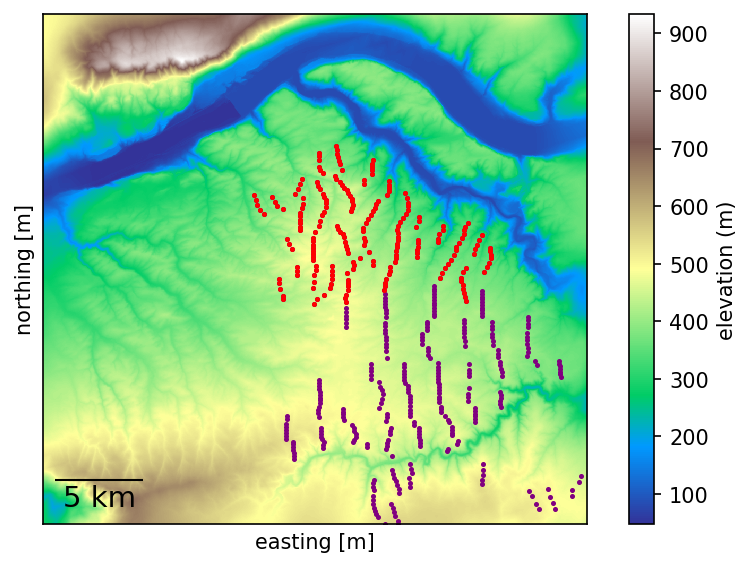
Nearby features, such as the Columbia River Gorge forms a gap in the mountain range and presents an environment that results in complex flow patterns. The region includes a few wind farms. In especial, in this case we model the turbines present in the Biglow Canyon wind farm. An overview of the region considered in shown in Fig. 9, as well as nearby turbines.
Fig. 9 Overview of the complex terrain region near the WFIP2 site. The red dots are turbines from the Biglow Canyon wind farm; purple dots are turbines from nearby farms.
The goal of this study is to assess boundary-coupled SOWFA capabilities with a challenging case that contains several features together. The period of interest investigated is November 21, 2016. In this day, there were significant mountain waves present.
Here, the microscale is driven by mesoscale data from WRF fed as boundary conditions. To handle the mountain wave and gravity waves that form in the domain, we will use Rayleigh damping layers at the top boundary. The turbines from the Biglow Canyon wind farm are modelled using the actuator disk model.
Relevance to wind energy
Complex terrain case including turbines
Gravity waves are excited due to the terrain and conditions during the period of interest
MMC Techniques Demonstrated
Application of boundary-coupled cases using different codes (WRF for mesoscale; SOWFA for microscale) on a complex terrain scenario
Terrain-conforming boundary coupling with WRF requires careful alignment of data
The setup of this case involves a few different aspects we will go over in this section. More details of the case can be seen in the setup scripts of the microscale execution in SOWFA, linked below.
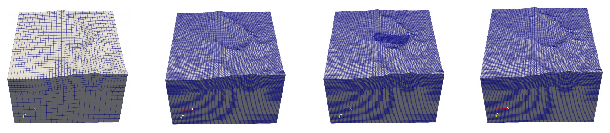
The domain extents are shown in Fig. 9. We model a 30 x 30 km region. In order to map terrain-conforming mesoscale data to a terrain-conforming microscale domain, we create the grid in steps, illustrated in Fig. 10. First, we create a coarse LES grid that conforms to a geometry STL file, thus having the bottom boundary points matching the locations of the bottom boundary points from the mesoscale domain. After that step, the quantities are mapped from the mesoscale domain onto the microscale. Next, the grid is refined to an appropriate level for turbulence-resolving large-eddy simulation. Additional local refinement regions around turbines can be added to the domain if desired. Finally, the higher resolution grid is conformed to the high-resolution STL geometry once again. The last step conforms the grid to the topographic details that were missing from the first step. This approach is needed to ensure WRF data exist at all point at the bottom boundary for proper mapping.
Fig. 10 Grid strategy for the microscale simulations. Bottom boundary shown on top. First image shows a coarse grid conformed to terrain, matching mesoscale grid size; In the second image, refinements bring the grid to desired resolution; Third image, local refinement zones can be included around turbines; And in the last image, the higher resolution grid is conformed again to the high-resolution terrain geometry.
The goal is to include all 217 turbines from the Biglow Canyon wind farm on the microscale simulation. Refinement zones near the turbines are needed to better capture their wake. Fig. 11 shows a close-up view of the turbines and their refinements upstream and downstream the rotor.
Note
Example of automatic generation of refinement zones around turbines is demonstrated in a Jupyter notebook available at the SOWFA repository.
Fig. 11 Close-up view of the turbines at the Biglow Canyon wind farm. The shaded area represents a grid refinement surrounding the turbine. The refinements are usually aligned with the wind direction to capture the turbine’s wake.
Gravity waves usually appear in the period of interest. The waves are organized perturbations in the vertical velocity component. The perturbation can reflect at the top boundary and create spurious turbulence that leads to numerical instabilities and unphysical flowfield. To prevent that, we use Rayleigh damping zones near the top of the domain.
Cell perturbation methods are also used to trigger turbulence development and reduce fetch extents. In the preliminary results presented in this page, no perturbation methods are used, but the setup will be updated in the near future including them.
The WFIP2/Biglow Canyon case analysis is still being performed. This page will be updated upon completion.
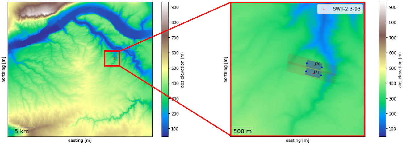
Preliminary mesoscale-coupled simulations are presented in terms of flowfield visualization. The domains considered are shown in Fig. 12. The left panel is the whole domain described previously and the right panel contain a smaller region where we focus on two Siemens SWT-2.3-93 turbines.
Fig. 12 Zoomed domain with two Siemens turbines considered for preliminary results.
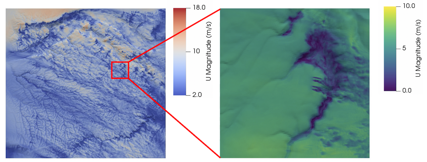
The results of the domains shown above is presented next in Fig. 13. The left panel shows the wind speed over the large domain. Note the large fetch needed for turbulence development. The fetch is large in this case because no temperature perturbation has been applied. On the right-hand-side panel, a smaller zoomed-in domain with two turbines is shown. Although the grid in this case was relatively coarse, the turbine wakes can be clearly seem.
Fig. 13 Wind speed over the 30x30 km region of interest around the Biglow Canyon wind farm shown in the left panel. The right panel shows a snapshot for the smaller case containing two Siemens turbines.