This study examines a well-observed cold air pool (CAP) case from the second Wind Forecast Improvement Project (WFIP2).
Cold pools frequently occur in the complex terrain of this region, the Columbia River Gorge.
These events can be challenging to forecast for numerical weather prediction models due to small-scale atmospheric processes.
Here, we focus on a 10-day case study from 10-20 January 2017 because the time period encapsulates the full evolution of the CAP: development, persistence, and erosion.
A main focus of the study is to better understand the horizontal variability in meteorological and turbulence quantities during the CAP lifecycle.
To highlight these aspects of the event, we use ground-based in-situ and remote sensing measurements, in addition to the Weather Research and Forecasting (WRF) model.
We conduct high-resolution mesoscale (sub-kilometric) simulations using various planetary boundary layer (PBL) parameterizations.
The impact of the WRF PBL parameterizations on the modeled horizontal variability in meteorological and turbulence quantities will be presented.
Of particular interest is the performance of a three-dimensional PBL scheme that was recently implemented into WRF [Kosović et al., 2020, Eghdami et al., 2022, Juliano et al., 2022].
Additional details about this WFIP2 CAP study may be found in the original report by Arthur et al. [2022].
Relevance to Wind Energy
Informs low wind energy production scenarios in complex terrain during stable conditions
Highlights the need for more comprehensive PBL parameterizations to reduce wind prediction errors
MMC Technique Demonstrated
Application of a novel three-dimensional PBL scheme developed by NCAR to improve wind forecasting
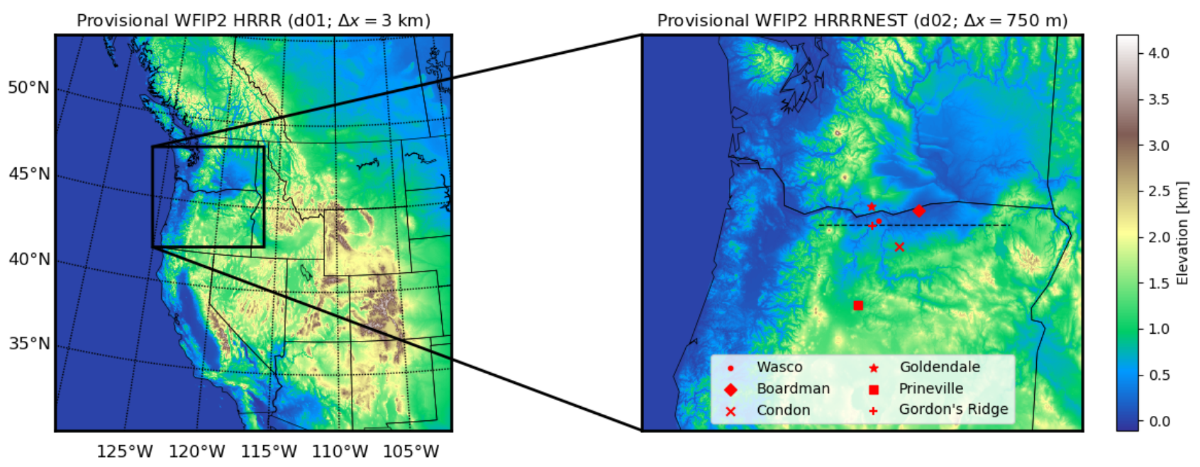
This study utilizes two nested domains (one-way coupling) with ∆x,y = 3 km in the outer domain (d01) and 750 m in the inner domain (d02) (Fig. 5).
Domains 1 and 2 are both mesoscale domains, i.e., they both use a PBL parameterization.
The vertical grid is consistent across both domains with 50 levels and ∆z ≈ 15 m near the surface before stretching above.
Fig. 5 WRF domain setup for the 10-day CAP event: HRRR (d01) and HRRRNEST (d02) are shown in the left and right panels. In d02, the locations of various WFIP2 measurement sites are shown by the red markers. This image is reproduced from Arthur et al. [2022] (their Fig. 1).
The outer domain is initialized using the operational Rapid Refresh (RAP) model.
Reforecast simulations using the HRRR and HRRRNEST setup are conducted every 12 hours from 00 UTC 10 January 2017 through 12 UTC 19 January 2017 and integrated for 24 hours each.
The WRF configuration (including input, boundary, and namelist files) is available through the U.S. Department of Energy (DOE) Data Archive and Portal (DAP; http://a2e.energy.gov/data).
Here, we focus on two WRF configurations from Arthur et al. [2022], which are listed in Table 1.
Table 1 Turbulence mixing/horizontal diffusion treatments for Cases #1, 2, and 3. This table is reproduced from Arthur et al. [2022] (their Table 1).
Case #
d01
d02
1
MYNN PBL w/ 2D Smag. along coordinate surfaces
MYNN PBL w/ 2D Smag. along coordinate surfaces
2
MYNN PBL w/ 2D Smag. in physical space
MYNN PBL w/ 2D Smag. in physical space
3
MYNN PBL w/ 2D Smag. in physical space
3D PBL w/ PBL Approx. in physical space
Attention
Case #1 is not emphasized in the present analysis because it is the same as Case #2, except it computes horizontal diffusion along coordinate surfaces. Our main intention here is to compare MYNN and 3D PBL when both compute horizontal diffusion in physical space.
The only difference between Cases #2 and 3 is the treatment of vertical turbulent mixing and horizontal diffusion on d02: Case #2 uses the MYNN PBL scheme for 1D (vertical) turbulent mixing and the Smagorinsky-approach for 2D (horizontal) diffusion, while Case #3 uses the 3D PBL scheme w/ PBL approximation to handle both vertical and horizontal turbulent mixing.
Details about additional sensitivity simulations related to both the horizontal diffusion method (physical space versus along coordinate surfaces), in addition to specific components of the 3D PBL parameterization, are provided in Arthur et al. [2022].
The surface-based observations from WFIP2 are freely available from the DOE DAP.
Please see Arthur et al. [2022] (their Table 2) for detailed information about the WFIP2 instruments used in this study.
The WRF input, boundary, and namelist files for each reforecast period are also available through the DOE DAP.
The WRF outputs generated from this study and used in the analysis are available from the authors upon reasonable request.
The WRF simulations are conducted using the Lawrence Livermore National Laboratory (LLNL) Livermore Computing (LC) resources.
Each WRF simulation is run every 12 hours for 24 hours of simulation time, resulting in a total of 20 simulations to cover the 10-day period.
Given the modest computing resources used (4 nodes x 36 cores = 144 processors) for the simulations, the wall clock to simulation time ratio is approximately 1.7 (40 hours wall clock to 24 hours simulation time).
The assessment performed in this study is catalogued on the A2e-MMC GitHub
An overview of the vertical structure of the cold pool event during the 10-day period as observed at the Wasco site is shown in Fig. 6.
Specifically, we show the evolution of the measured potential temperature and wind speed profiles, as well the model bias from Case #3, which generally performs better than Case #2 on the whole, as will be shown below.
Fig. 6 Measurements of (a) potential temperature and (c) wind speed at the Wasco WFIP2 site, in addition to the Case #3 model bias (b,d), for the 10-day CAP event. Results are shown for the first 12 hours (hours 3-15) of each reforecast period. This image is reproduced from Arthur et al. [2022] (their Fig. 2). Contours of observed temperature (units in degrees Celsius) are included in (a,b) for reference.
The CAP developed on 13 January, as indicated by a deepening of the near-surface layer of relatively cool temperatures and calm winds.
These conditions persisted for about 6 days until 18 January, at which point relatively strong winds and warmer temperatures eroded the strong near-surface inversion.
During the CAP period, model Case #3 tends to have a cool bias adjacent to the surface and a warm bias above ~200 m above ground level (AGL).
Wind biases are generally positive in the lowest few 100s of m AGL and negative around 500-1000 m AGL.
The model biases are amplified during the cold pool erosion period, which has been reported previously as a challenge in this region [Olson and Coauthors, 2019, Wilczak and Coauthors, 2019].
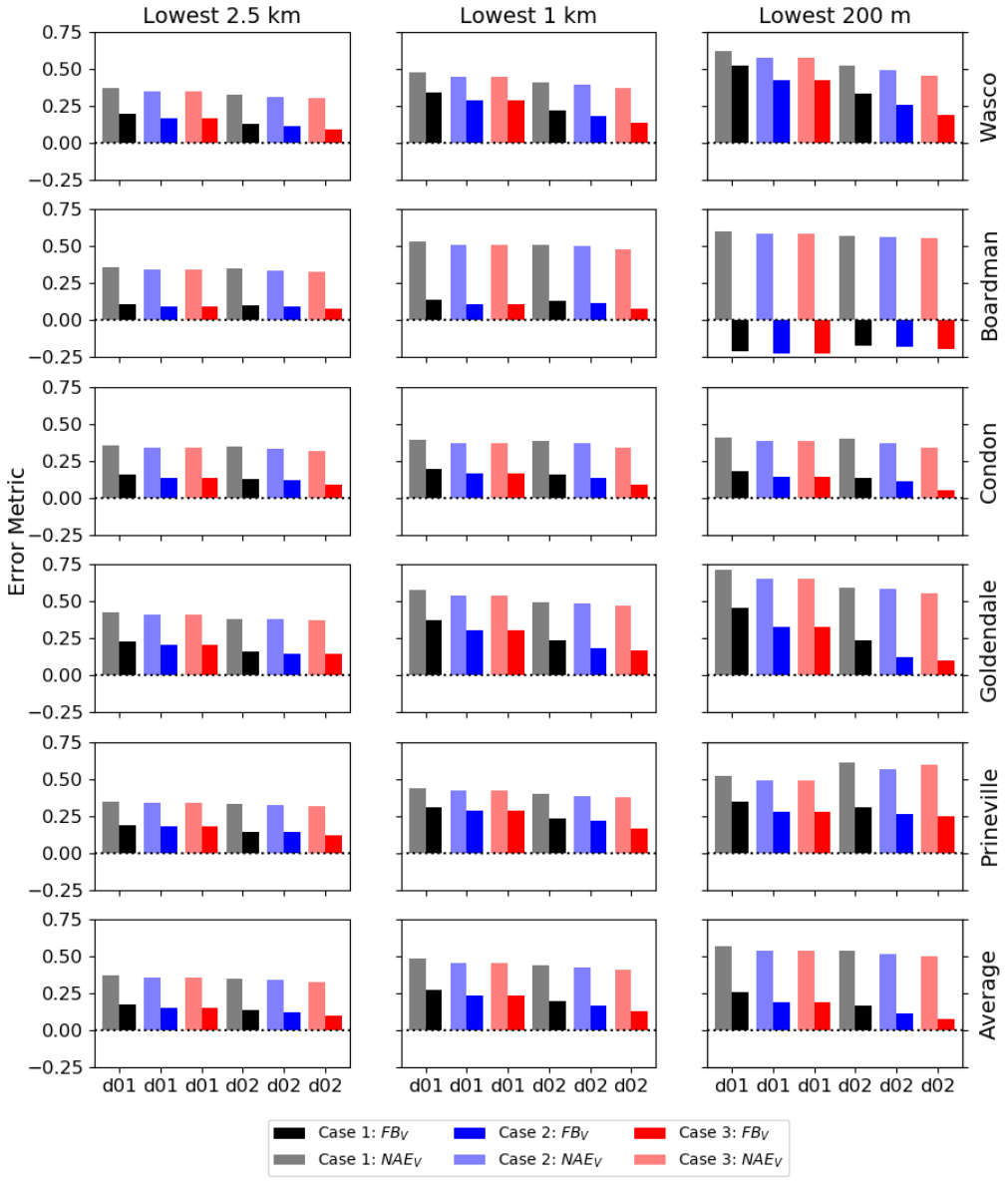
Fig. 7 Event-averaged wind speed error metrics for each case shown in Table 1. Results are shown for the (left) lowest 2.5 km AGL, (middle) lowest 1 km AGL, and (right) lowest 200 m AGL. Each observational site is shown individually, followed by an average over all five sites. The first 12 hours of each reforecast (i.e., hours 3-15) are used in the calculation. Note that because Cases #2 and 3 have the same setup on d01, their error metrics on d01 are identical. This image is reproduced from Arthur et al. [2022] (their Fig. 4).
Two error metrics are computed for several WFIP2 sites across the entire 10-day CAP event: fractional bias (FB) and normalized absolute error (NAE). FB is computed as:
where the overbar denotes an average over all available observations. \(FB_{\phi}\) captures whether, on average, the model over- or underestimates the observation, while \(NAE_{\phi}\) captures the average magnitude of the difference between the model and observation.
The error metrics for event-averaged wind speed are summarized in Fig. 7.
Comparing Cases #2 and 3 , it is evident that the more comprehensive turbulence mixing parameterization (Case #3, 3D PBL) tends to produce the most accurate forecast at nearly every site and for both error metrics.
An important component of any turbulence kinetic energy (TKE)-based PBL parameterization is the computation of the eddy diffusivity, which dictates the strength of turbulent mixing and depends upon the magnitude of TKE.
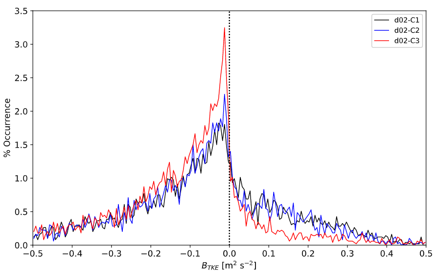
To evaluate the performance of MYNN (Case #2) and 3D PBL (Case #3) with respect to TKE prediction, the bias is computed at Gordon’s Ridge and shown in Fig. 8.
Fig. 8 Histograms of the TKE model bias values. Model bias is calculated for d02 using the first 12 hours of each reforecast (i.e., hours 3-15) and using observed TKE from the profiling lidar at Gordon’s Ridge. Details about the TKE bias computation may be found in Arthur et al. [2022]. This image is reproduced from Arthur et al. [2022] (their Fig. 8).
The overall TKE model biases tend to be negative (underestimation in TKE) for both Cases #2 and 3.
However, the positive biases are reduced substantially when using the 3D PBL parameterization.
The reason for this improvement in TKE prediction is primarily due to the different length scale formulations between MYNN and 3D PBL.
Further details regarding the observed and modeled turbulence characteristics from this CAP event are reported in Arthur et al. [2022].
Robert S. Arthur, Timothy W. Juliano, Bianca Adler, Raghavendra Krishnamurthy, Julie K. Lundquist, Branko Kosović, and Pedro A. Jiménez. Improved Representation of Horizontal Variability and Turbulence in Mesoscale Simulations of an Extended Cold-Air Pool Event. Journal of Applied Meteorology and Climatology, 61(6):685–707, June 2022. doi:10.1175/JAMC-D-21-0138.1.
Haupt2019
Sue Ellen Haupt, Branko Kosovic, William Shaw, Larry K. Berg, Matthew Churchfield, Joel Cline, Caroline Draxl, Brandon Ennis, Eunmo Koo, Rao Kotamarthi, Laura Mazzaro, Jeffrey Mirocha, Patrick Moriarty, Domingo Muñoz-Esparza, Eliot Quon, Raj K. Rai, Michael Robinson, and Gokhan Sever. On Bridging a Modeling Scale Gap: Mesoscale to Microscale Coupling for Wind Energy. Bulletin of the American Meteorological Society, August 2019. doi:10.1175/BAMS-D-18-0033.1.
B. Kosović, P. Jimenez Munoz, T. W. Juliano, A. Martilli, M. Eghdami, A. P. Barros, and S. E. Haupt. Three-Dimensional Planetary Boundary Layer Parameterization for High-Resolution Mesoscale Simulations. Journal of Physics: Conference Series, 1452(1):012080, January 2020. doi:10.1088/1742-6596/1452/1/012080.
J. B. Olson and Coauthors. Improving wind energy forecasting through numerical weather prediction model development. Bull. Amer. Meteor. Soc., 100:2201–2220, 2019.
J. M. Wilczak and Coauthors. The second wind forecast improvement project (wfip2): observational field campaign. Bull. Amer. Meteor. Soc., 100:1701–1723, 2019.