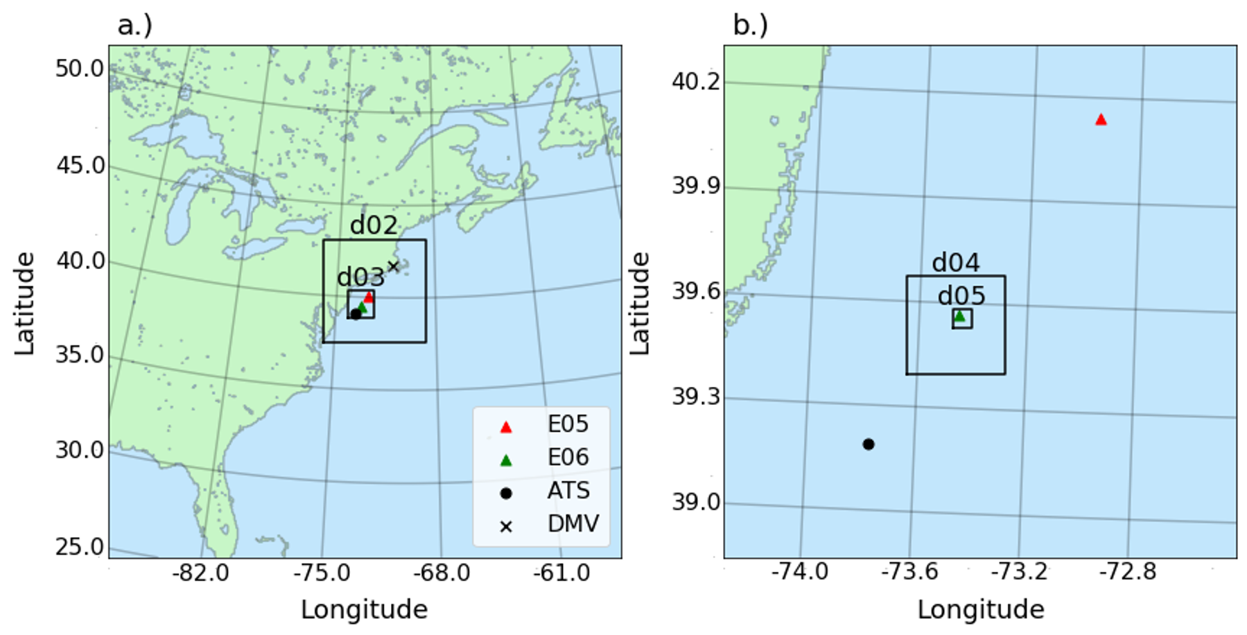
This study utilizes two floating lidars deployed by the New York State Energy and Research Development Authority (NYSERDA) in the New York Bight.
These buoys (E05 and E06 in Fig. 19) have been deployed within wind energy leased areas with data freely available from the summer of 2019 through present.
The period of interest for this particular case is from April 4, 2020 at 06Z to April 6, 2020 at 06Z in which a persistent low level jet is observed at both buoys.
A targeted simulation period for the LES domains is on April 6 from 00Z to 06Z.
The goal if this study is to assess how model sensitivities to factors such as sea surface temperature (SST), sea surface roughness, and land use change across scales.
This is done by performing an ensemble of mesoscale-to-microscale simulations, calculating ensemble statistics and various metrics on each domain, and comparing how these metrics change between the mesoscale domains and microscale domains.
Fig. 19 Locations of the NYSERDA floating lidar buoys and wind energy leased areas. (Image courtesy of Mike Optis.)
Relevance to Wind Energy
Informs forecasting/operational modeling of wind farm conditions as to what surface forcings are important and at which scale they need to be modeled
Informs resource assessment strategies in the offshore environment
Impacts on Uncertainty Quantification (UQ)
MMC Techniques Demonstrated
Ensemble mesoscale modeling and assessing best performers + model sensitivity
Stochastic cell perturbation method with Eckert scaling on LES domains
This setup utilizes 5 inline one-way nests with ∆x,y starting from 6.25 km and nesting down with ratios of 5:1 to 10 m (Fig. 20).
Domains 1 and 2 are both mesoscale domains while domains 3-5 are LES.
The vertical grid is consistent across all domains with 131 levels.
Below 400 m, the average ∆z is 10 m.
Above this point, ∆z stretches to around 420 m at model top.
Fig. 20 WRF domain configuration for (a) domains 1-3 and (b) domains 3-5.
Additionally, a setup script is available in which the case will be setup automatically on a user’s local environment.
This allows for easy recreation of the model simulations from this study.
Meso-to-LES cases are computationally expensive. When all 5 domains are running, Cheyenne is able to get 20 minutes of simulation time in roughly 10 hours of wall clock. Thus, the LES simulation output is the combined output of 12 individual runs that are restarted every 20 minutes of simulation time resulting in a total of 4 hours of simulation.
This study utilizes several auxiliary SST datasets (Fig. 21) and surface parameterizations to determine model sensitivity of the low-level jet (LLJ) to surface temperature and surface characteristics such as roughness.
The SST datasets vary in resolution and fidelity which can be easily seen by examining the gradients of SST.
When on the LES domains, the overall differences are generally constrained to subtle gradients over the domain with a different mean SST.
Fig. 21 Auxiliary SST datasets utilized within this study.
The additional tests that are run include using WRF’s SST skin parameterization, a 1-D ocean mixed-layer model (OMLM), implementing a shallow water roughness parameterization, and changing the land use dataset.
WRF’s SST skin parameterization [Zeng and Beljaars, 2005] prognostically calculates diurnal fluctuations in SST.
The 1-D OMLM model [Zi-Qian and An-Min, 2012] adjusts SST based on the gradients of SST and other variables such as wind speed.
Lastly, the shallow water roughness scheme [Jiménez and Dudhia, 2018] calculates over-water roughness based on bathymetry (for depths between 10 and 100 m).
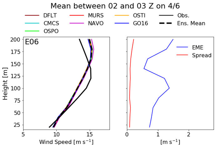
Results from the mesoscale simulations show that despite changing the SST dataset, there is very little change in the mean profile of the LLJ (Fig. 22 a) resulting in very low spread (Fig. 22 b).
Ensemble mean error also shows a consistent pattern between the SST datasets and auxiliary datasets with the lowest error near the surface and between the observed jet nose and simulated jet nose.
Fig. 22 Vertical profiles of (a) mean wind speed and (b) ensemble mean error and spread for the mesoscale runs (d02) for the SST cases.
The same can be said for the auxiliary surface feature tests (Fig. 23) in which the vertical profiles of wind speed are very similar for each case resulting in low spread.
Fig. 23 Vertical profiles of (a) mean wind speed and (b) ensemble mean error and spread for the mesoscale runs (d02) for the auxiliary tests.
Attention
LES simulations are ongoing. This page will be updated upon completion.
Patrick Hawbecker, William Lassman, Jeff Mirocha, Raj K. Rai, Regis Thedin, Matthew Churchfield, Sue Ellen Haupt, and Colleen Kaul. Offshore Sensitivities across Scales: A NYSERDA Case Study. In 102nd American Meteorological Society Annual Meeting. 2022.
Jayaraman2022
Balaji Jayaraman, Eliot Quon, Jing Li, and Tanmoy Chatterjee. Structure of Offshore Low-Level Jet Turbulence and Implications to Mesoscale-to-Microscale Coupling. Journal of Physics: Conference Series, 2265(2):022064, May 2022. doi:10.1088/1742-6596/2265/2/022064.
Pedro A Jiménez and Jimy Dudhia. On the need to modify the sea surface roughness formulation over shallow waters. Journal of Applied Meteorology and Climatology, 57(5):1101–1110, 2018.
Xubin Zeng and Anton Beljaars. A prognostic scheme of sea surface skin temperature for modeling and data assimilation. Geophysical Research Letters, 2005.