This study is centered around the offshore environment near the FINO1 meteorological tower and the Alpha Ventus
offshore wind farm. FINO stands for “Forschungsplattformen in Nord- und Ostsee”, which is German, and translates
to “Research platforms in the North Sea and Baltic Sea” in English. An overview of the region around the FINO1
tower is shown in Fig. 14, and the FINO1 website can be found here.
Fig. 14 Overview of the region where the Alpha Ventus wind farm is located.
The goal of this study is to compare different MMC techniques and identify each individual weaknesses and strengths.
More specifically, the focus is on a comparison across different information transfer locations and software usage.
We use different coupling strategies among different codes and compare mean quantities, as well as turbulence by
means of correlation analysis.
Relevance to wind energy
Low roughness of the offshore environment and lack of terrain produces low-turbulence conditions
Coupling methods can produce artifacts that, when present, can be the dominant features
There are no set of guidelines on how mesoscale coupling should be performed in the offshore environment
MMC Techniques Demonstrated
Application of profile assimilations technique for internally coupled cases
Application of boundary-coupled cases on different codes, namely SOWFA and WRF-LES
Initial setup based on the SWiFT case. It consists of 88 vertical levels and uses ERA5 reanalysis data, and MYJ
PBL scheme. Details of the mesoscale setup and how to obtain ERA5 driving data is detailed in the notebook listed
below.
Internal-Coupled Mesoscale to Microscale: WRF-Mesoscale to SOWFA-LES
This case demonstrates the coupling of a mesoscale model to a separate microscale model. In this case, the mesoscale
model is WRF, and the microscale model is SOWFA. This case demonstrates what we call “internal coupling.”
Specifically, the profile assimilation technique is used to drive the mean microscale conditions to a reference state
given by the mesoscale model through the use of a background source term forcing on microscale momentum and potential
temperature. This forcing is a smooth function of z and t only (i.e., it assumes horizontal homogeneity). With internal
coupling we retain the lateral periodicity of typical ABL large-eddy simulations.
An advantage of the internal-coupled case is that there is no fetch region where the turbulence is developing.
Because of that, we can use the whole domain for analysis, with the underlying assumptions that the flowfield is
horizontally homogeneous. The horizontal mean of the LES matches mesoscale profiles, so this method should be used only
when the horizontal gradients in the mesoscale flow are small. The resolved turbulence in the microscale is not forced
with the mesoscale forcing term, but it does react to the mean conditions the forcing imposes.
Boundary-Coupled Mesoscale to Microscale: WRF-Mesoscale to SOWFA-LES
Like with the previous case, this case also demonstrates coupling a mesoscale model, WRF, to a standalone microscale model, SOWFA.
But in this case, the coupling location is through boundary conditions.
We drive the microscale flow through two-dimensional boundary data extracted from the full WRF three-dimensional
fields every N seconds. On lateral boundaries, these data consist of velocity vector and potential temperature
information. At the lower surface, the data are surface roughness and sea-surface temperature or heat flux
information. Because we are extracting mesoscale data in which no turbulence is directly resolved, we then have to
apply some form of perturbations to initiate resolved-scale turbulence in the microscale, and in this case, we
use temperature cell perturbations. Although less simple than the internal-coupled method, the boundary-coupled method is more general in that horizontal
inhomogeneity is possible. However, a disadvantage is that there is a significant fetch region where turbulence has to come to a
properly formed state.
Boundary-Coupled Mesoscale to Microscale: WRF-Mesoscale to WRF-LES, Mann Synthetic Turbulence
This last case couples a mesoscale model with a microscale model all within one code, WRF. The finest simulation nests
are treated with LES, whereas the coarser nests use typical mesoscale turbulence modeling. Coupling of information is through
nest boundaries, so similar to the previous WRF to SOWFA boundary-coupled case, but all within a single code.
Here, we simulate the microscale flow using the one-way offline approach in multiple nested domains in the WRF framework.
This nesting approach allows downscale grid spacing from mesoscale, O(1) km, to microscale, O(1) m. A perturbation field of velocity or
temperature is applied along the inflow boundaries of the microscale domain to spin up the turbulence. For example, the velocity
perturbation field was prepared using Mann’s synthetic turbulence method. The turbulence field was applied to the
boundary-layer height on the lateral side of the domain in 10 seconds interval.
Boundary-Coupled Mesoscale to Microscale: WRF-Mesoscale to WRF-LES, Cell Perturbation Method
Attention
This work is still in progress.
Boundary-Coupled Mesoscale to Microscale: WRF-Mesoscale to WRF-LES, Control
The microscale simulations in both WRF and SOWFA uses mesoscale data produced by WRF. WRF mesoscale case, on the other hand, uses the aforementioned ERA5 reanalysis data.
The microscale runs, in special those executed using SOWFA, require an additional significant I/O overhead for sampling data. In this study, planes of data were saved at a temporal frequency of 1 second during the period of interest.
The flow over the period of interest is generally from the Northwest. In methods in which the mesoscale data is fed as boundary conditions, we expect a fetch region where the turbulence is still developing. For the results show in this section, we exclude such fetch from our analysis as it does not represent physical, resolved turbulence.
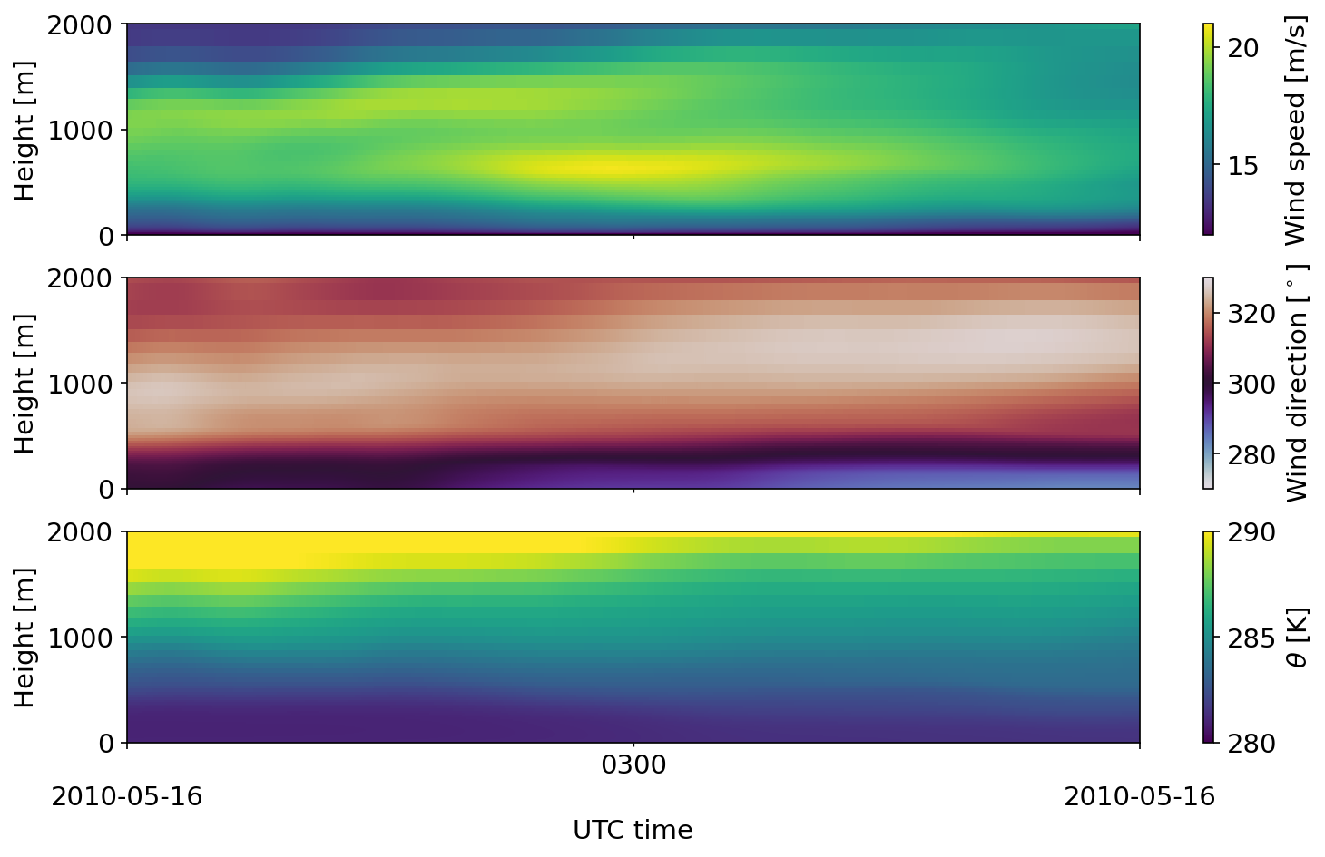
A time-height plot of the mesoscale driving conditions for the MMC techniques explored is shown in Fig. 15.
Fig. 15 Time-height data from the mesoscale model used to drive the microscale simulations.
View/Download the Assessment Notebooks
The assessment performed in this study is catalogued via Jupyter Notebooks on the A2e-MMC
GitHub
The period of interest for this case is 4-hour interval between 01Z and 04Z on May 16th, 2010, as indicated in Fig. 15. Shown next are some vertical profiles at every 30 minutes during the period of interest– Fig. 16. For each MMC technique investigated, observation data is plotted alongside observation data. Note that in the earlier part of the period of interest, the observation data show some waked effects between 80 and 100 m.
Fig. 16 Ten-minute mean vertical profile comparison across the different codes and techniques. Dots represent observation data.
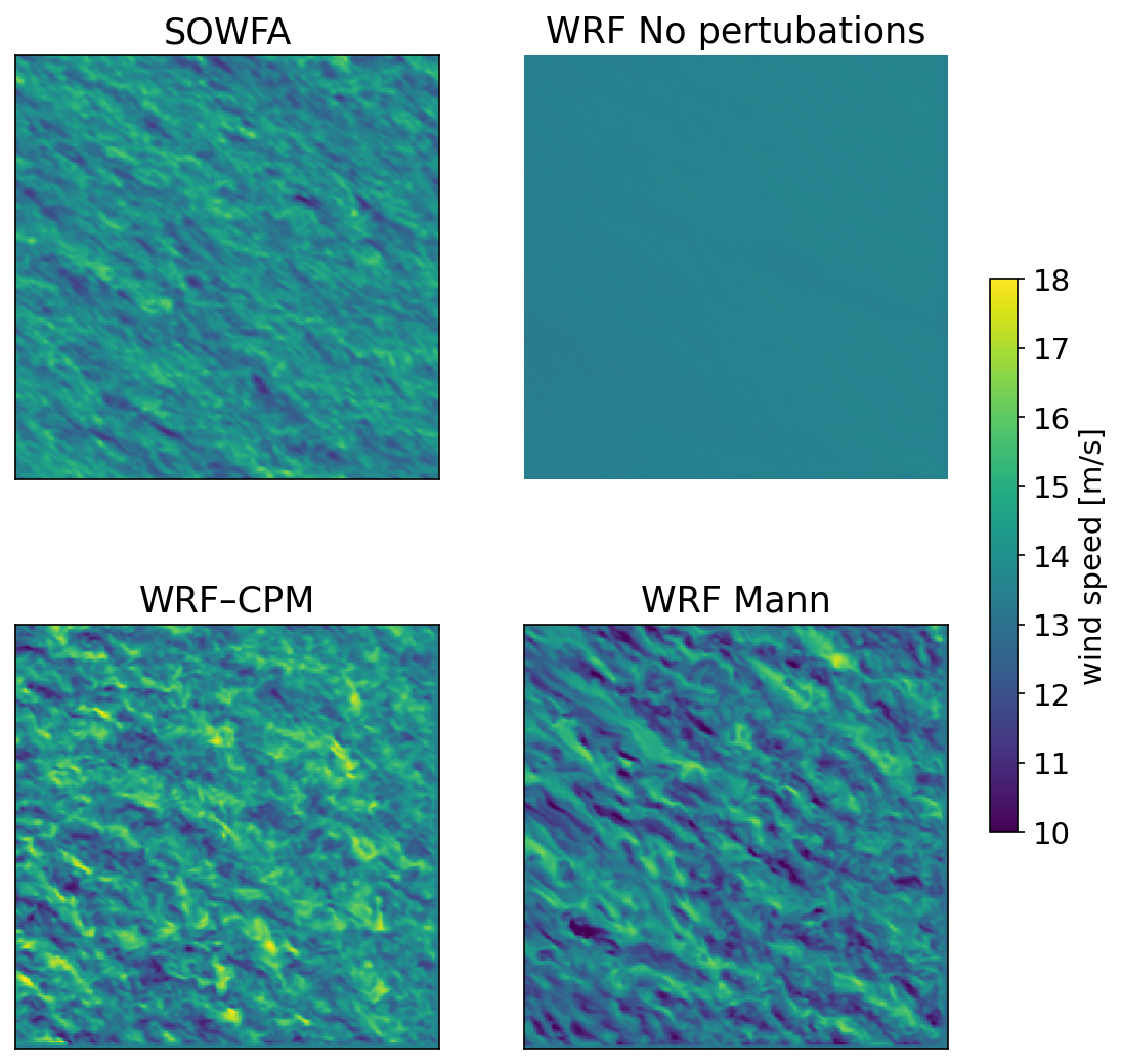
A snapshot of the instantaneous flowfield is shown in Fig. 17. The figure shows a 3-by-3 km subdomain region focused on the Southeast corner of the domain, leaving out the fetch region.
Fig. 17 Instantaneous snapshot of the flowfield as calculated by the different methods.
Even thought average quantities and instantaneous flowfield appears similar (with the exception of the control case), a spectral analysis reveals differences in the methods. Power spectral density plots are shown in Fig. 18.
Fig. 18 Power spectral density results for all methods for all 3 components of the velocity field, at 80 m.
The SOWFA case matches the energy content of the observations. Both WRF Mann and the cell perturbation method have higher similar, higher energy content. The energy of the streamwise component is larger than the others, as expected. The control case exhibted little turbulence and the power spectral density plots clearly shows the lack of energy in the flow.
Attention
SOWFA boundary-coupled simulations are still being performed. This page will be updated upon completion.
Attention
Spatial correlation analysis is currently underway for WRF cases. This section will be updated with the results from all codes upon completion.
Regis Thedin, Eliot Quon, Matthew Churchfield, and Paul Veers. Investigations of Correlation and Coherence in Turbulence from a Large-Eddy Simulation. Wind Energ. Sci. Discuss., 2022. doi:10.5194/wes-2022-71.